Definition: A linear function is a function whose points form a straight line when graphed. The equation takes the form ![]() or
or ![]() . A linear function is a polynomial of degree 1.
. A linear function is a polynomial of degree 1.
Arithmetic Sequences
An arithmetic sequence is an example of a function whose points lie on a straight line.
In general, the domain of an arithmetic sequence is the set of natural numbers ![]() . The range is the set of terms in the sequence.
. The range is the set of terms in the sequence.
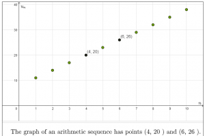
When graphed, the points in the sequence lie on a straight line. There are no intermediate points, so we don’t draw a line through these points.

The general term for the sequence graphed here is ![]() .
.
Review how to find the general term for an arithmetic sequence from the graph here.
From Arithmetic Sequences to Linear Functions
The structure of the formula for arithmetic sequences and linear functions is identical. Instead of variables ![]() (place value) and
(place value) and ![]() (term value), we use the generic labels
(term value), we use the generic labels ![]() and
and ![]() . Instead of
. Instead of ![]() for common difference – the amount the sequence increases each term – we use
for common difference – the amount the sequence increases each term – we use ![]() for ‘slope’ or ‘gradient’ which is the amount the line goes up for one whole unit right.
for ‘slope’ or ‘gradient’ which is the amount the line goes up for one whole unit right.
When studying linear functions in general, we assume the domain is the set of all possible numbers, that is, every value on the ![]() axis. We say “
axis. We say “![]() is a member of the set of real numbers”, and we write
is a member of the set of real numbers”, and we write ![]() . The range is also all possible numbers. To express the range we write
. The range is also all possible numbers. To express the range we write ![]() .
.
Check out the similarities and differences in this applet:
Applications
A linear function can be used to apply math to any data set where there is a steady increase or decrease, or an approximately steady increase or decrease. Linear functions are also used extensively in the study of calculus.
Example 1: Pay
When a person is being paid by the hour, they might work 1, 2, 3, …10 hours (like an arithmetic progression), however if they work 3.25 hours they will be paid for the ‘0.25’. Here is the example of the appliance repair technician from unit 5.
The linear function that fits this data set is ![]() , or
, or ![]() if you prefer to use letters that represent the Cost (C) and the number of hours (h). You can type this equation in the input bar to see the linear function. The cost of 3 hours and 15 minutes work (that is 3.25 hours) is
if you prefer to use letters that represent the Cost (C) and the number of hours (h). You can type this equation in the input bar to see the linear function. The cost of 3 hours and 15 minutes work (that is 3.25 hours) is ![]() .
.
Example 2: Scatter plot
Sometimes the scatter plot of a data set suggests a linear function. In this case we calculate what is known as a ‘line of best fit’. Click the image below to the mathisfun web page that describes this process.
Example 3: Calculus
The study of calculus is the study of how things change. On the polynomial curve below you can see how the steepness of the curve changes as you drag the dynamic point along the curve. We use the relatively simple tangent line to give us more information about the relatively complicated curve.
In this unit we learn how to understand and calculate the ‘slope’ of a linear function; we learn three different ways to express a linear function, we learn about horizontal and vertical lines, parallel and perpendicular lines, and finally, we learn how to compute the ![]() and the
and the ![]() intercepts of linear functions. These skills are universal to learning how to apply linear functions in the three examples given above. (Examples 2 and 3 are beyond the scope of the grade 10 course).
intercepts of linear functions. These skills are universal to learning how to apply linear functions in the three examples given above. (Examples 2 and 3 are beyond the scope of the grade 10 course).

